Molecular Orbital (MO) Theory

 

Introduction

 

     Individual atoms have atomic orbitals that represent the electron around a single nucleus.  When two or more atoms interact, their valence electrons are delocalized across the overlapping orbitals.  One way to describe the movement of these electrons is using molecular orbitals. Molecular orbitals describes the location of electrons throughout an entire molecule. The molecular orbitals of molecules are the combinations of atomic orbitals that represent the electron density of the entire molecule. 

 

     Molecular orbitals are calculated using the linear combination method of atomic orbitals. The size and shape of molecular orbitals are determined by adding and subtracting the individual atoms' atomic orbitals in such a way as to produce the distribution of individual molecular electrons across the entire molecule. Molecular orbitals, in essence, describe the state of the molecule--that is the energy and density probability of the electrons the molecule.

 

History

 

     In 1916, G. N. Lewis developed a theory of bonding which included the idea of pairs of electrons being shared equally or unequally between two atoms, completing an electron shell of two (for the in-most shell) or eight. According to the theory developed by Lewis, shared pairs of electrons were called bonding electrons and electrons not part of the bonding were called lone pairs.

 

     Langmuir, in 1919, extended Lewis's model by theorizing molecules of the same number of electrons, which he called isostere, have basically the same electronic structure and properties (such as N_{2 and} CO₂).

 

     With the help of Linear Combination of Atomic Orbitals, Robert Mulliken's insight into the world of orbitals in 1932, and Friedrich Hund's development of atomic structure, molecular orbital theory was developed. In 1938, the first correct calculation of a molecular orbital wavefunction was executed by Charles Coulson on the hydrogen molecules.  By the 1950s, molecular orbitals were completely defined by wavefunctions and the Hamiltonian.

 

Schrodinger Equation/Linear Combination of Atomic Orbitals (LCAO)

 

Schrodinger Equation

     The Schrodinger equation gives a wave function in the stationary state for a system

 

Ψ is the wave function, h is Planck's constant and m is the mass of the particle. For a hydrogen atom, it is easy to solve this equation, because it only has one electron. Solving the equation gives exact expressions for the energy levels and the wave functions. The square of the wave function gives the probability of finding an electron at a specific position in space. We can therefore obtain a mathematical expression to the areas in which we will expect to find an electron. The wave functions are called hydrogen atomic orbitals. 

 

Quantum Numbers

     Quantum numbers describe values of conserved quantities in the dynamics of a quantum system. It is a set of integers which determine the properties of an electron which determine its state. This model describes electrons using three quantum numbers (the forth quantum number, magnetic spin, m_s, describes the state of the electron but is not used to describe atomic orbitals): 

1. The principal quantum number: n - the individual energy level. Can have the values n=1, 2, 3... 
2. The angular momentum number: ℓ - can take any value from 0 to n-1. 
3. The magnetic quantum number: m_ℓ - can take any value from – ℓ to ℓ  

To describe the state of an electron we need a set of those three numbers (n, ℓ,m). By convention, we call the magnetic quantum numbers by the letters that represent the shape of the orbital, outlined by the chart below.

 

ℓ	letter
0	s
1	p
2	d
3	f
4	g

 

     We can then describe a state of an electron with n=1 and ℓ=0 by 1s, n=2 and ℓ=0 by 2s etc.

 

     Since an exact solution can only be found for atoms with one electron (H, He⁺,Li²⁺) the atomic orbitals found for a hydrogen atom are used to approximate solutions for more complex systems.  The Schrodinger equation becomes a three-body problem when there is more than one electron, due to the interaction between each electron and the nucleus and interaction between the electrons.  Three-body problems cannot be solved analytically, thus the numerical algorithms are used to find approximate solutions. 

 

Linear Combination of Atomic Orbitals

     The linear combination of atomic orbitals is a method of approximating molecular electronic wave functions from atomic orbitals. This method generates an orbital that is delocalized over the whole molecule. The approximation generated from this method is used to calculate properties of this molecule.

 

     Generally, the approximate wave function of an electron in a molecule will be obtained from some linear combination of the wave functions from each atom separately. In this example, the molecular wave function is a sum of two 1s wave functions:

 

     Ψ(t)=AΨ₁(t)+BΨ₂(t)

 

     If A>B, then the function will have more of the A wave character, and the electron would be more likely to be found around the nucleus of A. This property is reflected in the apparent shape of the generated molecular orbitals.

 

Geometry of Orbitals

 

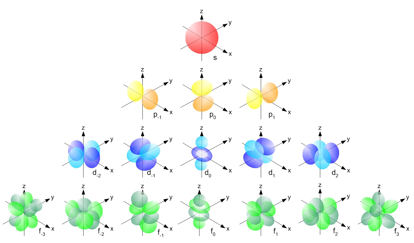
     Four different atomic orbitals exist in MO theory, s, p, d, and f. All orbitals have their own shape and energy associated with them.  There is one s orbital that can hold up to two electrons.  Three p orbitals exist that can hold up to two electrons each, thus six electrons in total.  There are five d orbitals that can hold ten electrons total, and seven f orbitals that can hold fourteen electrons in total.  The different shapes and orientations of the orbitals can be seen by the diagram below. 

 

     Each orbital, as mentioned, has specific energies.  The order of the orbitals from least energy to highest energy is as follows: 1s, 2s, 2p, 3s, 3p, 4s, 3d, 4p, 5s, 4d, 5p, 6s, 4f, 5d, 6p, 7s, 5f, 6d, 7p.  It is common practice to write how many electrons are in each orbital when describing atoms.  For example Neon would be written as 1s² 2s² 2p⁶ and Potassium would be written as 1s² 2s² 2p⁶ 3s² 3p⁶ 4s¹.  Electrons first fill the atomic orbitals which have the lowest energy.

 

     When creating molecules through the bonding of atoms, atomic orbitals overlap to form molecular orbitals.  It is important to remember only atomic orbitals similar energy interact to a significant degree.  When the two atomic orbitals from similar atomic orbitals overlap, two extreme molecular orbitals form:  a bonding molecular orbital and an antibonding molecular orbital, which will be explained in the next section.   

 

Representation via Diagram

 

     Instead of considering how electrons are delocalized over an entire molecule, the molecular orbital concept approximates the location and energy of an electron donated by an atom by only considering atoms directly adjacent to the atom of interest. Thus, molecular orbitals are derived by combining the atomic orbitals of the atom of interest and the atoms directly adjacent. 

 

     For molecular orbitals, electrons participate in one of two interactions: sigma or pi bonds. Sigma bonds occur when electrons are shared along the inter-nuclear (z) axis of two atoms (i.e. the line drawn directly between them). When electrons are shared through sigma bonds, hybridization of that atom’s atomic orbitals occurs. This is commonly known as a ‘single bond’ for purposes of determining molecular structure. Electrons are shared in pi bond interactions when a double bond is formed. A pi bond is formed ‘on top of’ a sigma bond and, unlike a sigma bond, is not a formal ‘sharing’ of electrons. Instead, a pi bond is formed when electrons of two or more atoms’ in-phase p orbitals interact with each other, allowing any electrons in these orbitals to be shared parallel to the inter-nuclear axis. 

 

     Because the formation of these molecular orbitals must be energetically favorable to take place, an energy diagram is the most intuitive way to represent their formation. Naturally, a molecular orbital will be lower on the energy scale while the individual atomic orbitals will be relatively higher. By connecting the atomic orbitals to the molecular orbitals, we can represent the flow of electrons and the formation of the bond. While molecular orbital diagrams represent how atoms form bonds, they also represent how bonds are broken. For each molecular orbital that is formed a subsequent anti-bonding orbital is formed as well. As shown in the example diagram, an anti-bonding orbital is at a higher energy level than the bonding orbital that is formed. Anti-bonding orbitals are described using an asterisk (*). For instance, anti-bonding sigma bonds are referred to as 'sigma-star,' and pi anti-bonding orbitals are referred to as 'pi-star.' Electrons are excited to the anti-bonding orbital when large amounts of energy and put into the system. When there is more energy in the system, it becomes favorable for electrons to use this energy to move to the anti-bonding orbital subsequently dissolving the bond between the two atoms.

 

     Drawing molecular orbital diagrams is relatively simple. The two atoms involved in the bonding are drawn on either side, while the orbitals being formed are drawn between the atoms. Lines are drawn between orbitals to represent the movement, or potential movement of electrons.

These diagrams are an effective way to represent the energy levels of bonds in some complex molecules. For instance, the molecular orbital diagram of methane is given below:

Here, we can see the formation of four molecular orbitals resulting from the sharing of the carbon atom’s three p orbitals, its one s orbital, and the four s orbitals of the hydrogen atoms. Once electrons ‘fall’ into molecular orbitals, they are considered delocalized—meaning that they are not held by one specific atom. The different molecular orbitals that are formed have different energies; however, this does not mean that the individual C-H bonds have different energies. Instead, all eight electrons are shared throughout the molecule (which, in effect, is the molecular orbital representation of the electrons not using the hybrid orbital approximation). Molecular orbitals are how we can describe the electron density around the central atom. The physical appearance of these orbitals reflects the linear combination of the atomic orbitals invloved. Note that the number of molecular orbitals that are formed is half the number of the electrons shared in the molecule (2 electrons occupy each orbital). Combinations of lower energy orbitals results in a molecular orbital with a lower overall energy.

 

Molecular Vs. Hartree Orbitals

 

     As previously mentioned, molecular orbitals are essentially the linear combination of atomic orbitals of the various atoms throughout the molecule. These orbitals in MO theory are derived using the linear combination of atomic orbitals method (LCAO) in which the atomic orbitals involved in the formation of the molecular orbitals are 'averaged' together to yield a combined orbital that reflects properties of all atomic orbitals combined in the process. This process is relatively simple--however it does not take into account other forces that may act on an electron involved in bonding. The Hartree-Fock method takes into account several other factors that effect the position of an electron in a molecule, which are listed below:

 

     1. Considers how other electrons effect the position of the observed electron

     2. Creates 'effective fields' by averaging the effects other electrons might have on the location of another electron

 

These considerations make the Hartree-Fock method much more accurate at describing the behavior of electrons at high energy levels--where the effect of electron shielding is the greatest.  In effect, the Hartree-Fock method is a more comprehensive way of describing the position-probability of high-energy electrons in both atomic and molecular orbitals because it considers the effects of other electrons on the formation of orbitals. 

 

Exploration of Molecular Orbitals Using Modern Computing Programs

 

     Modern computer programs allow chemists to calculate the shape of molecular orbitals relatively easily. In essence, these programs perform the complex calculations involved in the LACO method and plot the values of the function across the molecule. This can be a helpful tool for determining molecular reactivity. For instance, we can look at the molecular orbital diagram for ethene generated by SPARTAN:  

 

 

We can now generate the highest occupied molecular orbital (HOMO) to view how electrons with the highest energy are distributed throughout the molecule:

 

 

As you can see, electron density for the HOMO is distributed evenly throughout the molecule because both carbon atoms are equal in their tendency to attract the electron density (electronegativity) and have identical AO configurations. The electron density is concentrated above and below the inter-nuclear axis, indication that the HOMO is a pi bond.

 

Now we can generate the the HOMO for vinyl alcohol (CH₂CHOH) to see how the molecular orbitals accommodate the additional hydroxyl group:

 

 

As you can see, the molecular orbital calculations suggest that electron density will be directed toward the newly added oxygen atom. This is a consequence of the added complexity of the AOs of oxygen as well as its tendency to attract electrons away from its neighboring carbon atom. The pi bond character between the two carbon atoms can still be observed, but the overall density appears to be reduced due to the additional AOs of oxygen.

 

     Using computer programs such as these provide valuable insight to the state of molecular systems. 

 

Questions

 

1. Molecular orbitals

     a. are the same as atomic orbitals

     b. are formed from the overlap of atomic orbitals

     c. are not related to atomic orbitals

     d. are called s, p, d, and f

     e. both a and d

 

2. The energies of bonding molecular orbitals is

     a. Always greater than the atomic orbitals

     b. Always less than the atomic orbitals

     c. Always equal to the atomic orbitals

     d. Always equal to or less than the atomic orbitals

     e. Always equal to or greater than to the atomic orbitals

 

3. Solutions to the Schrodinger Equation...

     a. Are achievable for any atom

     b. Are the quantum numbers n, l, and m

     c. Are only real number integers

     d. b & c

     e. a & b     

 

 

Answers:

1. b

2. b

3. b

 

References

 

University of Califonia Davis. (2012). Single electron orbitals. [ [Web Graphic]]. Retrieved from http://chemwiki.ucdavis.edu/Physical_Chemistry/Quantum_Mechanics/Atomic_Theory/Electrons_in_Atoms/Electronic_Orbitals 

 

Mulliken, R. S. (n.d.). The path to molecular orbital theory. Retrieved from http://www.iupac.org/publications/pac/pdf/1970/pdf/2401x0203.pdf

 

Blauch, David N. Virtual Chemistry Experiments. Retrieved from

http://www.chm.davidson.edu/vce/molecularorbitals/

 

Oxtoby, David W.; Gillis, H. Pat; Campion, Alan; Principles of Modern Chemistry, 7th Edition. Cengage Learning: 2011.